Bézier curve

Cubic Bézier curve

A Bézier curve is a parametric curve frequently used in computer graphics and related fields. Generalizations of Bézier curves to higher dimensions are called Bézier surfaces, of which the Bézier triangle is a special case.

In vector graphics, Bézier curves are used to model smooth curves that can be scaled indefinitely. "Paths," as they are commonly referred to in image manipulation programs^{[note 1]} are combinations of linked Bézier curves. Paths are not bound by the limits of rasterized images and are intuitive to modify. Bézier curves are also used in animation as a tool to control motion.^{[note 2]}

Bézier curves are also used in the time domain, particularly in animation and interface design, e.g., a Bézier curve can be used to specify the velocity over time of an object such as an icon moving from A to B, rather than simply moving at a fixed number of pixels per step. When animators or interface designers talk about the "physics" or "feel" of an operation, they may be referring to the particular Bézier curve used to control the velocity over time of the move in question.

Bézier curves were widely publicized in 1962 by the French engineer Pierre Bézier, who used them to design automobile bodies. The curves were first developed in 1959 by Paul de Casteljau using de Casteljau's algorithm, a numerically stable method to evaluate Bézier curves.

Applications

Computer graphics

Bézier path in Adobe Illustrator

Bézier curves are widely used in computer graphics to model smooth curves. As the curve is completely contained in the convex hull of its control points, the points can be graphically displayed and used to manipulate the curve intuitively. Affine transformations such as translation, and rotation can be applied on the curve by applying the respective transform on the control points of the curve.

Quadratic and cubic Bézier curves are most common; higher degree curves are more expensive to evaluate. When more complex shapes are needed, low order Bézier curves are patched together. This is commonly referred to as a "path" in programs like Adobe Illustrator or Inkscape. These poly-Bézier curves can also be seen in the SVG file format. To guarantee smoothness, the control point at which two curves meet must be on the line between the two control points on either side.

The simplest method for scan converting (rasterizing) a Bézier curve is to evaluate it at many closely spaced points and scan convert the approximating sequence of line segments. However, this does not guarantee that the rasterized output looks sufficiently smooth, because the points may be spaced too far apart. Conversely it may generate too many points in areas where the curve is close to linear. A common adaptive method is recursive subdivision, in which a curve's control points are checked to see if the curve approximates a line segment to within a small tolerance. If not, the curve is subdivided parametrically into two segments, 0 ≤ t ≤ 0.5 and 0.5 ≤ t ≤ 1, and the same procedure is applied recursively to each half. There are also forward differencing methods, but great care must be taken to analyse error propagation. Analytical methods where a spline is intersected with each scan line involve finding roots of cubic polynomials (for cubic splines) and dealing with multiple roots, so they are not often used in practice.

Animation

In animation applications, such as Adobe Flash and Synfig, Bézier curves are used to outline, for example, movement. Users outline the wanted path in Bézier curves, and the application creates the needed frames for the object to move along the path. For 3D animation Bézier curves are often used to define 3D paths as well as 2D curves for keyframe interpolation.

Examination of cases

Linear Bézier curves

Given points P₀ and P₁, a linear Bézier curve is simply a straight line between those two points. The curve is given by

$\mathbf{B}(t)=\mathbf{P}_0 + t(\mathbf{P}_1-\mathbf{P}_0)=(1-t)\mathbf{P}_0 + t\mathbf{P}_1 \mbox{ , } t \in [0,1]$

and is equivalent to linear interpolation.

Quadratic Bézier curves

A quadratic Bézier curve is the path traced by the function B(t), given points P₀, P₁, and P₂,

$\mathbf{B}(t) = (1 - t)^{2}\mathbf{P}_0 + 2(1 - t)t\mathbf{P}_1 + t^{2}\mathbf{P}_2 \mbox{ , } t \in [0,1].$

It departs from P₀ in the direction of P₁, then bends to arrive at P₂ in the direction from P₁. In other words, the tangents in P₀ and P₂ both pass through P₁. This is directly seen from the derivate of the Bezier curve:

$\mathbf{B}'(t) = 2 (1 - t) (\mathbf{P}_1 - \mathbf{P}_0) + 2 t (\mathbf{P}_2 - \mathbf{P}_1) \,.$

A quadratic Bézier curve is also a parabolic segment.

TrueType fonts use Bézier splines composed of quadratic Bézier curves.

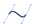
Cubic Bézier curves

Four points P₀, P₁, P₂ and P₃ in the plane or in three-dimensional space define a cubic Bézier curve. The curve starts at P₀ going toward P₁ and arrives at P₃ coming from the direction of P₂. Usually, it will not pass through P₁ or P₂; these points are only there to provide directional information. The distance between P₀ and P₁ determines "how long" the curve moves into direction P₂ before turning towards P₃.

The parametric form of the curve is:

$\mathbf{B}(t)=(1-t)^3\mathbf{P}_0+3(1-t)^2t\mathbf{P}_1+3(1-t)t^2\mathbf{P}_2+t^3\mathbf{P}_3 \mbox{ , } t \in [0,1].$

Since the lines $\mathbf{P}_0\mathbf{P}_1$ and $\mathbf{P}_2\mathbf{P}_3$ are the tangents of the Bézier curve at $\mathbf{P}_0$ and $\mathbf{P}_3$ , respectively, cubic Bézier interpolation is essentially the same as cubic Hermite interpolation.

Modern imaging systems like PostScript, Asymptote and Metafont use Bézier splines composed of cubic Bézier curves for drawing curved shapes.

Generalization

The Bézier curve of degree n can be generalized as follows. Given points P₀, P₁,..., P_n, the Bézier curve is

$\begin{align} \mathbf{B}(t) & = \sum_{i=0}^n {n\choose i}(1-t)^{n-i}t^i\mathbf{P}_i \\ & = (1-t)^n\mathbf{P}_0 + {n\choose 1}(1-t)^{n-1}t\mathbf{P}_1 + \cdots \\ & {} \quad \cdots + {n\choose n-1}(1-t)t^{n-1}\mathbf{P}_{n-1} + t^n\mathbf{P}_n,\quad t \in [0,1], \end{align}$

where $\scriptstyle {n \choose i}$ is the binomial coefficient.

For example, for n = 5:

$\begin{align} \mathbf{B}(t) & = (1-t)^5\mathbf{P}_0 + 5t(1-t)^4\mathbf{P}_1 + 10t^2(1-t)^3 \mathbf{P}_2 \\ & {} \quad + 10t^3 (1-t)^2 \mathbf{P}_3 + 5t^4(1-t) \mathbf{P}_4 + t^5 \mathbf{P}_5,\quad t \in [0,1]. \end{align}$

This formula can be expressed recursively as follows: Let $\mathbf{B}_{\mathbf{P}_0\mathbf{P}_1\ldots\mathbf{P}_n}$ denote the Bézier curve determined by the points P₀, P₁, ..., P_n. Then

$\mathbf{B}(t) = \mathbf{B}_{\mathbf{P}_0\mathbf{P}_1\ldots\mathbf{P}_n}(t) = (1-t)\mathbf{B}_{\mathbf{P}_0\mathbf{P}_1\ldots\mathbf{P}_{n-1}}(t) + t\mathbf{B}_{\mathbf{P}_1\mathbf{P}_2\ldots\mathbf{P}_n}(t)$

In other words, the degree-n Bézier curve is a linear interpolation between two degree-(n − 1) Bézier curves.

Terminology

Some terminology is associated with these parametric curves. We have

$\mathbf{B}(t) = \sum_{i=0}^n \mathbf{b}_{i,n}(t)\mathbf{P}_i,\quad t\in[0,1]$

where the polynomials

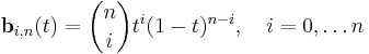
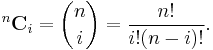
$\mathbf{b}_{i,n}(t) = {n\choose i} t^i (1-t)^{n-i},\quad i=0,\ldots n$

are known as Bernstein basis polynomials of degree n, defining t⁰ = 1 and (1 − t)⁰ = 1. The binomial coefficient, $\scriptstyle {n \choose i}$ , has the alternative notation,

$^n\mathbf{C}_i = {n \choose i} = \frac{n!}{i!(n-i)!}.$

The points P_i are called control points for the Bézier curve. The polygon formed by connecting the Bézier points with lines, starting with P₀ and finishing with P_n, is called the Bézier polygon (or control polygon). The convex hull of the Bézier polygon contains the Bézier curve.

The curve begins at P₀ and ends at P_n; this is the so-called endpoint interpolation property.
The curve is a straight line if and only if all the control points are collinear.
The start (end) of the curve is tangent to the first (last) section of the Bézier polygon.
A curve can be split at any point into two subcurves, or into arbitrarily many subcurves, each of which is also a Bézier curve.
Some curves that seem simple, such as the circle, cannot be described exactly by a Bézier or piecewise Bézier curve; though a four-piece cubic Bézier curve can approximate a circle, with a maximum radial error of less than one part in a thousand, when each inner control point (of offline point) is the distance $\textstyle\frac{4\left(\sqrt {2}-1\right)}{3}$ horizontally or vertically from an outer control point on a unit circle. More generally, an n-piece cubic Bézier curve can approximate a circle, when each inner control point is the distance $\textstyle\frac{4}{3}\tan(t/4)$ from an outer control point on a unit circle, where t is 360/n degrees, and n > 2.
The curve at a fixed offset from a given Bézier curve, often called an offset curve (lying "parallel" to the original curve, like the offset between rails in a railroad track), cannot be exactly formed by a Bézier curve (except in some trivial cases). However, there are heuristic methods that usually give an adequate approximation for practical purposes.
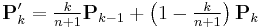
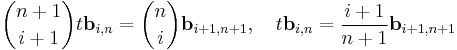
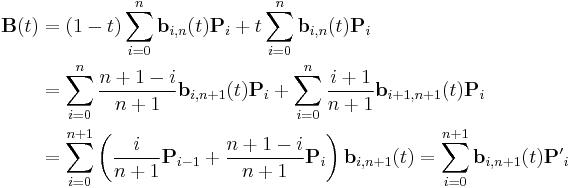
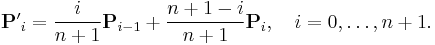
Every quadratic Bézier curve is also a cubic Bézier curve, and more generally, every degree n Bézier curve is also a degree m curve for any m > n. In detail, a degree n curve with control points P₀, …, P_n is equivalent (including the parametrization) to the degree n + 1 curve with control points P'₀, …, P'_{n + 1}, where $\mathbf P'_k=\tfrac{k}{n+1}\mathbf P_{k-1}+\left(1-\tfrac{k}{n+1}\right)\mathbf P_k$ .

Constructing Bézier curves

Linear curves

Animation of a linear Bézier curve, t in [0,1]

The t in the function for a linear Bézier curve can be thought of as describing how far B(t) is from P₀ to P₁. For example when t=0.25, B(t) is one quarter of the way from point P₀ to P₁. As t varies from 0 to 1, B(t) describes a straight line from P₀ to P₁.

Quadratic curves

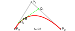
For quadratic Bézier curves one can construct intermediate points Q₀ and Q₁ such that as t varies from 0 to 1:

Point Q₀ varies from P₀ to P₁ and describes a linear Bézier curve.
Point Q₁ varies from P₁ to P₂ and describes a linear Bézier curve.
Point B(t) varies from Q₀ to Q₁ and describes a quadratic Bézier curve.


Construction of a quadratic Bézier curve		Animation of a quadratic Bézier curve, t in [0,1]

Higher-order curves

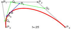
For higher-order curves one needs correspondingly more intermediate points. For cubic curves one can construct intermediate points Q₀, Q₁, and Q₂ that describe linear Bézier curves, and points R₀ & R₁ that describe quadratic Bézier curves:


Construction of a cubic Bézier curve		Animation of a cubic Bézier curve, t in [0,1]

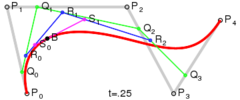
For fourth-order curves one can construct intermediate points Q₀, Q₁, Q₂ & Q₃ that describe linear Bézier curves, points R₀, R₁ & R₂ that describe quadratic Bézier curves, and points S₀ & S₁ that describe cubic Bézier curves:


Construction of a quartic Bézier curve		Animation of a quartic Bézier curve, t in [0,1]

(See also a construction of a fifth-order Bézier curve.)

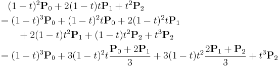
Degree elevation

A Bézier curve of degree n can be converted into a Bézier curve of degree n + 1 with the same shape. This is useful if software supports Bézier curves only of specific degree. For example, you can draw a quadratic Bézier curve with Cairo, which supports only cubic Bézier curves.

To do degree elevation, we use equality $\mathbf{B}(t) = (1-t)\mathbf{B}(t) + t\mathbf{B}(t)$ . Each component $\mathbf{b}_{i,n}(t)\mathbf{P}_i$ is multiplied by (1 − t) or t, thus increasing a degree by one. Here is the example of increasing degree from 2 to 3.

$\begin{align} & {} \quad (1 - t)^{2}\mathbf{P}_0 + 2(1 - t)t\mathbf{P}_1 + t^{2}\mathbf{P}_2 \\ & = (1 - t)^{3}\mathbf{P}_0 + (1 - t)^{2}t\mathbf{P}_0 + 2(1 - t)^{2}t\mathbf{P}_1 \\ & {} \qquad + 2(1 - t)t^{2}\mathbf{P}_1 + (1 - t)t^{2}\mathbf{P}_2 + t^{3}\mathbf{P}_2 \\ & = (1 - t)^{3}\mathbf{P}_0 + 3(1 - t)^{2}t\frac{\mathbf{P}_0 + 2\mathbf{P}_1}{3} + 3(1 - t)t^{2}\frac{2\mathbf{P}_1 + \mathbf{P}_2}{3} + t^{3}\mathbf{P}_2 \end{align}$

For arbitrary n we use equalities

${n+1 \choose i}(1-t)\mathbf{b}_{i,n} = {n \choose i} \mathbf{b}_{i,n+1}, \quad (1-t)\mathbf{b}_{i,n} = \frac{n+1-i}{n+1} \mathbf{b}_{i,n+1}$

${n+1 \choose i+1} t\mathbf{b}_{i,n} = {n \choose i} \mathbf{b}_{i+1,n+1}, \quad t\mathbf{b}_{i,n} = \frac{i+1}{n+1} \mathbf{b}_{i+1,n+1}$

$\begin{align} \mathbf{B}(t) & = (1-t)\sum_{i=0}^n \mathbf{b}_{i,n}(t)\mathbf{P}_i + t\sum_{i=0}^n \mathbf{b}_{i,n}(t)\mathbf{P}_i \\ & = \sum_{i=0}^n \frac{n+1-i}{n+1}\mathbf{b}_{i,n+1}(t)\mathbf{P}_i + \sum_{i=0}^n \frac{i+1}{n+1}\mathbf{b}_{i+1,n+1}(t)\mathbf{P}_i \\ & = \sum_{i=0}^{n+1} \left(\frac{i}{n+1}\mathbf{P}_{i-1} + \frac{n+1-i}{n+1}\mathbf{P}_i\right) \mathbf{b}_{i,n+1}(t) = \sum_{i=0}^{n+1} \mathbf{b}_{i,n+1}(t)\mathbf{P'}_i \end{align}$

introducing arbitrary $\mathbf{P}_{-1}$ and $\mathbf{P}_{n+1}$ .

Therefore new control points are ^[1]

$\mathbf{P'}_i = \frac{i}{n+1}\mathbf{P}_{i-1} + \frac{n+1-i}{n+1}\mathbf{P}_i,\quad i=0,\ldots, n+1.$

Polynomial form

Sometimes it is desirable to express the Bézier curve as a polynomial instead of a sum of less straightforward Bernstein polynomials. Application of the binomial theorem to the definition of the curve followed by some rearrangement will yield:

$\mathbf{B}(t) = \sum_{j = 0}^n {t^j \mathbf{C}_j}$

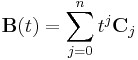
where

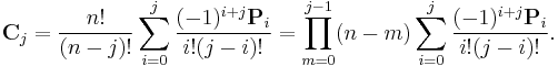
$\mathbf{C}_j = \frac{n!}{(n - j)!} \sum_{i = 0}^j \frac{(-1)^{i + j} \mathbf{P}_i}{i! (j - i)!} = \prod_{m = 0}^{j - 1} (n - m) \sum_{i = 0}^j \frac{(-1)^{i + j} \mathbf{P}_i}{i! (j - i)!} .$

This could be practical if $\mathbf{C}_j$ can be computed prior to many evaluations of $\mathbf{B}(t)$ ; however one should use caution as high order curves may lack numeric stability (de Casteljau's algorithm should be used if this occurs). Note that the empty product is 1.

Rational Bézier curves

Sections of conic sections represented exactly by rational Bézier curves

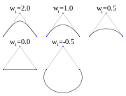
The rational Bézier curve adds adjustable weights to provide closer approximations to arbitrary shapes. The numerator is a weighted Bernstein-form Bézier curve and the denominator is a weighted sum of Bernstein polynomials. Rational Bézier curves can, among other uses, be used to represent segments of conic sections exactly.^[2]

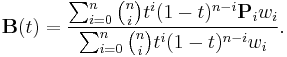
Given n + 1 control points P_i, the rational Bézier curve can be described by:

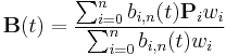
$\mathbf{B}(t) = \frac{ \sum_{i=0}^n b_{i,n}(t) \mathbf{P}_{i}w_i } { \sum_{i=0}^n b_{i,n}(t) w_i }$

or simply

$\mathbf{B}(t) = \frac{ \sum_{i=0}^n {n \choose i} t^i (1-t)^{n-i}\mathbf{P}_{i}w_i } { \sum_{i=0}^n {n \choose i} t^i (1-t)^{n-i}w_i }.$

Notes

↑ Image manipulation programs such as Inkscape, Adobe Photoshop, and GIMP.
↑ In animation applications such as Adobe Flash, Adobe After Effects, Microsoft Expression Blend, Blender, Autodesk Maya and Autodesk 3ds max.

References

↑ Farin, Gerald (1997), Curves and surfaces for computer-aided geometric design (4 ed.), Elsevier Science & Technology Books, ISBN 978 0 12249054 5
↑ Neil Dodgson (2000-09-25). "Some Mathematical Elements of Graphics: Rational B-splines". http://www.cl.cam.ac.uk/teaching/2000/AGraphHCI/SMEG/node5.html. Retrieved 2009-02-23.

Paul Bourke: Bézier Surfaces (in 3D), http://local.wasp.uwa.edu.au/~pbourke/geometry/bezier/index.html
Donald Knuth: Metafont: the Program, Addison-Wesley 1986, pp. 123–131. Excellent discussion of implementation details; available for free as part of the TeX distribution.
Dr Thomas Sederberg, BYU Bézier curves, http://www.tsplines.com/resources/class_notes/Bezier_curves.pdf
J.D. Foley et al.: Computer Graphics: Principles and Practice in C (2nd ed., Addison Wesley, 1992)

External links

Poly Bézier Curve Construction by jsDraw2D Graphics Library. The library is for JavaScript and is open source. The drawPolyBezier function in jsDraw2D implements the poly Bézier drawing algorithm.
Don Lancaster's Cubic Spline Library describes how to approximate a circle (or a circular arc, or a hyperbola) by a Bézier curve; using cubic splines for image interpolation, and an explanation of the math behind these curves.
Weisstein, Eric W., "Bézier Curve" from MathWorld.
Module for Bézier Curves by John H. Mathews
Multi-degree 2D Bézier Curve java applet - An interactive bezier curve applet implementing: adding and deleting control points, showing control polygon and convex hull, manipulating sampling amount and elevating degree without changing the curve.
PolyBezier – The Microsoft Win32 GDI API function, which draws Bézier curves in Windows graphic applications, like MS Paint.
Finding All Intersections of Two Bézier Curves. – Locating all the intersections between two Bézier curves is a difficult general problem, because of the variety of degenerate cases. By Richard J. Kinch.
SketchPad – A small program written in C and Win32 that implements the functionality to create and edit Bézier curves. Demonstrates also the use of de Casteljau's algorithm to split a Bézier curve.
Bézier Curves interactive demo using ActionScript and FlashPlayer – Includes Bézier curve and additional drawing/text tools.
Drawing Cubic Bézier Curves explained by using Flash Actionscript
3rd order Bézier Curves applet
Living Math Bézier applet
Living Math Bézier applets of different spline types, Java programming of splines in An Interactive Introduction to Splines
From Bézier to Bernstein Feature Column from American Mathematical Society
Bézier Curves demo using Flash Actionscript
Bézier Curves drawer using C/Opengl
Online experiments with the open source JavaScript library JSXGraph